Using dsmextra with ‘big data’: An example, with a note on covariate transformations
Phil J. Bouchet, David L. Miller, Jason Roberts, Laura Mannocci, Catriona M Harris, Len Thomas
Centre for Research into Ecological & Environmental Modelling, University of St Andrews2021-06-01
dsmextra-bigdata.RmdPreamble
This vignette demonstrates an application of dsmextra to a much larger dataset, which comprises 100 times as many segments (i.e., reference/calibration data points) as in the sperm whale example presented in the introductory vignette, and where the prediction area spans half the of the North Atlantic Ocean. We also briefly explore the effects of covariate transformations on extrapolation assessments.
Installation
The latest development version of dsmextra can be installed from GitHub (this requires the remotes package):
remotes::install_github("densitymodelling/dsmextra", dependencies = TRUE)
The code below loads required libraries and sets some general options.
#'---------------------------------------------
# Other required libraries
#'---------------------------------------------
library(dsmextra)     # Extrapolation toolkit for ecological models
library(raster)       # Geographic data analysis and modeling
library(tidyverse)    # Packages for data science
library(magrittr)     # Pipe operator

#'---------------------------------------------
# Set tibble options
#'---------------------------------------------
options(tibble.width = Inf) # All tibble columns shown
options(pillar.neg = FALSE) # No colouring negative numbers
options(pillar.subtle = TRUE)
options(pillar.sigfig = 4)

#'---------------------------------------------
# Set knitr options
#'---------------------------------------------
knitr::opts_chunk$set(echo = TRUE)
Overview
In the following, we show:
- How to run the
compute_nearbyfunction on ‘big’ data; - How covariate transformations, which are common in ecological research, may affect extrapolation assessments.
Data
The data for this example are stored in a list object called ziphius. These are fully described in Roberts et al. (2016) and Mannocci et al. (2017), and remain very similar in nature to the sperm whale data showcased in the introductory vignette.
str(ziphius, max.level = 2) # Inspect the list
## List of 2
##  $ segs   :'data.frame': 124995 obs. of  4 variables:
##   ..$ Depth                 : num [1:124995] 3.36 3.35 3.26 3.36 3.34 ...
##   ..$ DistToCanyonOrSeamount: num [1:124995] 2.45 3.66 4.47 4.71 4.56 ...
##   ..$ Chl1                  : num [1:124995] -1.11 -1.08 -1.03 -1.03 -1.05 ...
##   ..$ CurrentSpeed          : num [1:124995] -0.945 -0.97 -0.98 -0.976 -0.974 ...
##   ..- attr(*, "na.action")= 'omit' Named int [1:462] 512 910 1889 1987 1988 2075 2128 4189 6886 7200 ...
##   .. ..- attr(*, "names")= chr [1:462] "634" "1084" "2329" "2427" ...
##  $ rasters:Formal class 'RasterStack' [package "raster"] with 11 slots
As before, segs is a data.frame containing the segment data. Note, however, that coordinates for the segment mid-points are not available. Covariate layers are available as a RasterStack in ziphius$rasters.
| Depth | DistToCanyonOrSeamount | Chl1 | CurrentSpeed |
|---|---|---|---|
| 3.359937 | 2.449904 | -1.113293 | -0.9454697 |
| 3.349395 | 3.655052 | -1.075477 | -0.9704471 |
| 3.263835 | 4.467572 | -1.034892 | -0.9796294 |
| 3.355105 | 4.710572 | -1.029381 | -0.9759339 |
| 3.335688 | 4.556134 | -1.049879 | -0.9735497 |
| 3.246040 | 4.381402 | -1.092257 | -0.9678591 |
We consider four covariates likely to influence beaked whale density and distribution. Two of those are static (Depth and DistToCanyonOrSeamount), and two are dynamic (Chl1 and CurrentSpeed). For simplicity, dynamic covariates are taken as the yearly means across 12 monthly rasters.
#'---------------------------------------------
# Define projected coordinate system
#'---------------------------------------------
aftt_crs <- sp::CRS("+proj=aea +lat_1=38 +lat_2=30 +lat_0=34 +lon_0=-73 +x_0=0 +y_0=0 +datum=WGS84 +units=m +no_defs +ellps=WGS84 +towgs84=0,0,0")

#'---------------------------------------------
# Define environmental covariates of interest
#'---------------------------------------------
covariates.ziphius <- c("Depth", "DistToCanyonOrSeamount", "Chl1", "CurrentSpeed")
Analysis
Transforming covariates
Transforming explanatory covariates (for instance, to reduce the influence of outliers or make skewed distributions more symmetric) is common practice in ecological modelling. We can explore the effects of data transformations on extrapolation metrics by constructing two separate datasets, i.e., one with transformed values, the other not.
Within the ziphius list object, the data in segs have already been transformed, whereas those in rasters have not. In our case, \(log_{10}\) and square root transformations are applied to Depth/CurrentSpeed and to DistToCanyonOrSeamount, respectively. Remote-sensed chlorophyll-a values are frequently only used, and already provided, in \(log_{10}\) form - these will not be tempered with.
We apply the relevant (back)-transformations, as shown below:
segments.ziphius <- predgrid.ziphius <- list(transformed = NULL, untransformed = NULL)

#'---------------------------------------------
# Back-transform the segment-level covariate values
#'---------------------------------------------
segments.ziphius$transformed <- ziphius$segs
segments.ziphius$untransformed <- ziphius$segs %>%
  dplyr::mutate(Depth = 10^Depth) %>%
  dplyr::mutate(DistToCanyonOrSeamount = (DistToCanyonOrSeamount^2)*1000) %>%
  dplyr::mutate(CurrentSpeed = 10^CurrentSpeed)

#'---------------------------------------------
# Transform covariate rasters
#'---------------------------------------------
predgrid.ziphius$untransformed <- ziphius$rasters
predgrid.ziphius$transformed <- purrr::map(.x = seq_len(raster::nlayers(ziphius$rasters)),
                .f = ~{
                  r <- ziphius$rasters[[.x]]
                  if(names(ziphius$rasters)[.x]%in%c("Depth", "CurrentSpeed")) r <- log10(r)
                  if(names(ziphius$rasters)[.x]=="DistToCanyonOrSeamount") r <- sqrt(r/1000)
                  names(r) <- names(ziphius$rasters)[.x]
                  r
                }) %>% raster::stack(.)
The final prediction grids (i.e., target data) can now be put together.
predgrid.ziphius$untransformed <- raster::as.data.frame(predgrid.ziphius$untransformed,
                                                         xy = TRUE, na.rm = TRUE)
predgrid.ziphius$transformed <- raster::as.data.frame(predgrid.ziphius$transformed,
                                                       xy = TRUE, na.rm = TRUE)
Quantifying extrapolation
ExDet values can be calculated on both the transformed and untransformed datasets.
ziphius.extrapolation <- list(transformed = NULL, untransformed = NULL)

ziphius.extrapolation$untransformed <-
  compute_extrapolation(samples = segments.ziphius$untransformed,
                        covariate.names = covariates.ziphius,
                        prediction.grid = predgrid.ziphius$untransformed,
                        coordinate.system = aftt_crs)

ziphius.extrapolation$transformed <-
  compute_extrapolation(samples = segments.ziphius$transformed,
                        covariate.names = covariates.ziphius,
                        prediction.grid = predgrid.ziphius$transformed,
                        coordinate.system = aftt_crs)
Transformations appear to have a minimal effect on extrapolation results, as the extent of univariate extrapolation is identical amongst datasets. Current speed is the only covariate responsible for combinatorial extrapolation in the untransformed case, albeit to a minute degree.
purrr::map(.x = ziphius.extrapolation, .f = summary)
## $transformed
##
##
## Table: Extrapolation
##
## Type          Count         Percentage
## ------------  ------------  ------------
## Univariate    22067         20.01
## Analogue      88187         79.99
## -----------   -----------   -----------
## Total         110254        100
##
##
## Table: Most influential covariates (MIC)
##
## Type          Covariate                Count         Percentage
## ------------  -----------------------  ------------  ------------
## Univariate    Chl1                     21818         20
## Univariate    CurrentSpeed             239           0.22
## Univariate    DistToCanyonOrSeamount   7             0.0063
## Univariate    Depth                    3             0.0027
## -----------   -----------              -----------   -----------
## Total                                  22067         20
##
## $untransformed
##
##
## Table: Extrapolation
##
## Type            Count         Percentage
## --------------  ------------  ------------
## Univariate      22067         20.01
## Combinatorial   2             0
## -----------     -----------   -----------
## Sub-total       22069         20.02
## -----------     -----------   -----------
## Analogue        88185         79.98
## -----------     -----------   -----------
## Total           110254        100
##
##
## Table: Most influential covariates (MIC)
##
## Type            Covariate                Count         Percentage
## --------------  -----------------------  ------------  ------------
## Univariate      Chl1                     21818         20
## Univariate      CurrentSpeed             239           0.22
## Univariate      DistToCanyonOrSeamount   7             0.0063
## Univariate      Depth                    3             0.0027
## -----------     -----------              -----------   -----------
## Sub-total                                22067         20
## -----------     -----------              -----------   -----------
## Combinatorial   CurrentSpeed             2             0.0018
## -----------     -----------              -----------   -----------
## Sub-total                                2             0.0018
## -----------     -----------              -----------   -----------
## Total                                    22069         20
Comparing covariates
Running the code on the untransformed data:
compare_covariates(extrapolation.type = "both",
                   extrapolation.object = ziphius.extrapolation$untransformed,
                   n.covariates = NULL,
                   create.plots = TRUE,
                   display.percent = TRUE)
## Preparing the data ...## Computing ...## ## Creating summaries ...## Done!
##
##
## Extrapolation   Minimum                                       n_min  Maximum                                             n_max
## --------------  -------------------------------------------  ------  --------------------------------------------------  ------
## Univariate      Depth                                             3  Depth, DistToCanyonOrSeamount, Chl1, CurrentSpeed   22067
## Combinatorial   Depth                                             0  Depth, DistToCanyonOrSeamount                       2
##                 DistToCanyonOrSeamount                            0  Depth, DistToCanyonOrSeamount, Chl1                 2
##                 Chl1                                              0  Depth, DistToCanyonOrSeamount, CurrentSpeed         2
##                 CurrentSpeed                                      0  Depth, DistToCanyonOrSeamount, Chl1, CurrentSpeed   2
##                 Depth, CurrentSpeed                               0  -                                                   -
##                 DistToCanyonOrSeamount, Chl1                      0  -                                                   -
##                 DistToCanyonOrSeamount, CurrentSpeed              0  -                                                   -
##                 Chl1, CurrentSpeed                                0  -                                                   -
##                 DistToCanyonOrSeamount, Chl1, CurrentSpeed        0  -                                                   -
## Both            Depth                                             3  Depth, DistToCanyonOrSeamount, Chl1, CurrentSpeed   22069
Running the code on the transformed data:
compare_covariates(extrapolation.type = "both",
                   extrapolation.object = ziphius.extrapolation$transformed,
                   n.covariates = NULL,
                   create.plots = TRUE,
                   display.percent = TRUE)
## Preparing the data ...## Computing ...## ## Creating summaries ...## Done!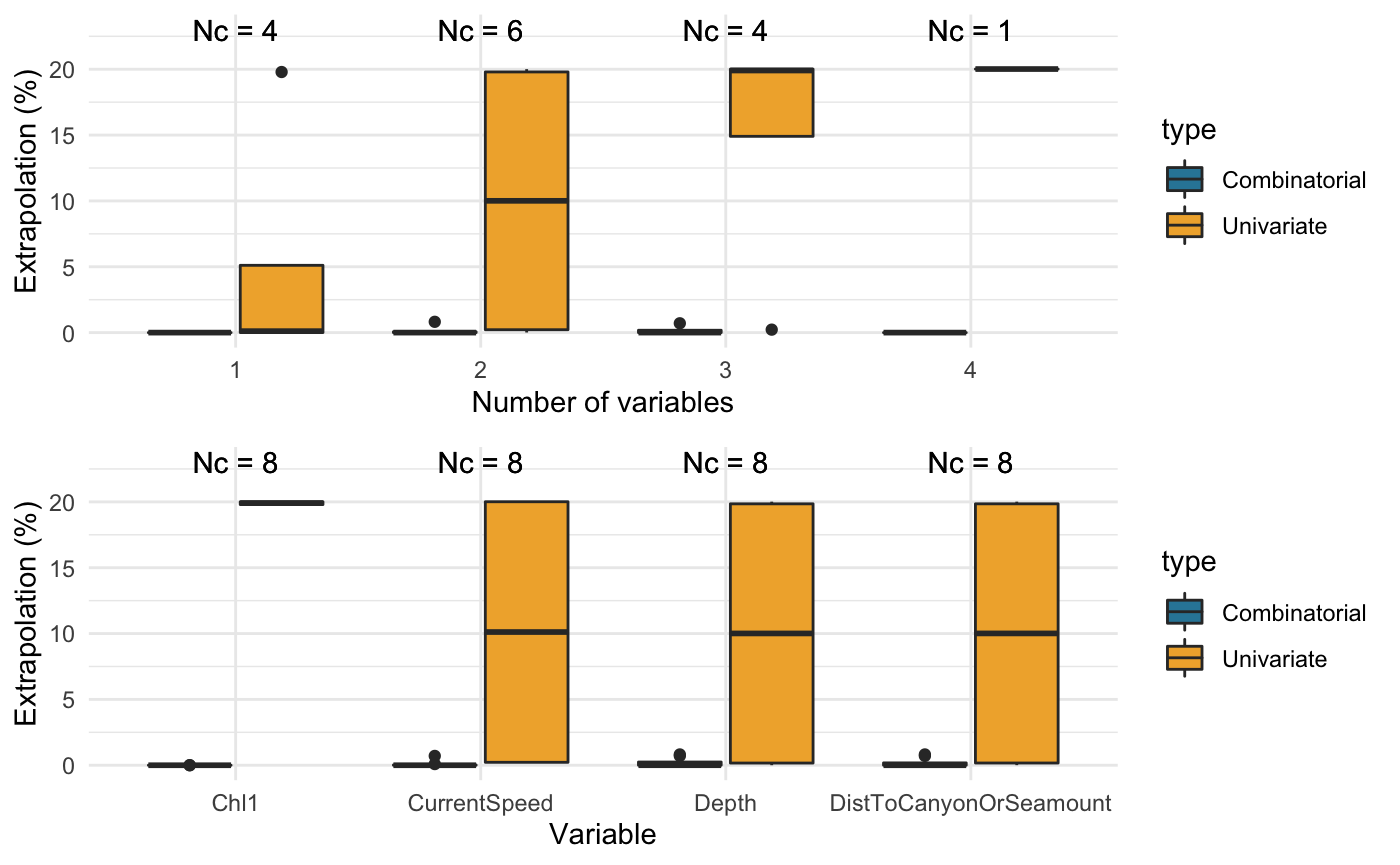
##
##
## Extrapolation   Minimum                                              n_min  Maximum                                             n_max
## --------------  --------------------------------------------------  ------  --------------------------------------------------  ------
## Univariate      Depth                                                    3  Depth, DistToCanyonOrSeamount, Chl1, CurrentSpeed   22067
## Combinatorial   Depth                                                    0  Depth, DistToCanyonOrSeamount                       905
##                 DistToCanyonOrSeamount                                   0  -                                                   -
##                 Chl1                                                     0  -                                                   -
##                 CurrentSpeed                                             0  -                                                   -
##                 DistToCanyonOrSeamount, Chl1                             0  -                                                   -
##                 DistToCanyonOrSeamount, CurrentSpeed                     0  -                                                   -
##                 Chl1, CurrentSpeed                                       0  -                                                   -
##                 Depth, Chl1, CurrentSpeed                                0  -                                                   -
##                 DistToCanyonOrSeamount, Chl1, CurrentSpeed               0  -                                                   -
##                 Depth, DistToCanyonOrSeamount, Chl1, CurrentSpeed        0  -                                                   -
## Both            Depth                                                    3  Depth, DistToCanyonOrSeamount, Chl1, CurrentSpeed   22067
Finding nearby data
The whatif function from the Whatif package (Gandrud et al. 2017), which is called internally by compute_nearby, may not run on very large datasets. While this was not an issue with the sperm whale case study in the introductory vignette, the beaked whale dataset is several orders of magnitude larger.
data("spermwhales")
size.df <- tibble(species = c("Sperm whales", "Beaked whales"), size = c(format(prod(nrow(spermwhales$segs),
    nrow(spermwhales$predgrid)), nsmall = 0, big.mark = ","), format(prod(nrow(ziphius$segs),
    nrow(predgrid.ziphius$transformed)), nsmall = 0, big.mark = ",")))
knitr::kable(size.df, format = "pandoc")
| species | size |
|---|---|
| Sperm whales | 5,015,465 |
| Beaked whales | 13,781,198,730 |
To circumvent this problem, the whatif.opt function sets the calculations performed by whatif to run on partitions of the data instead, for greater efficiency. whatif.opt can be called internally within compute_nearby by using two additional arguments, namely:
-
max.size: Threshold above which partitioning will be triggered. -
no.partitions: Number of required partitions.
In practice, a run of compute_nearby begins with a quick assessment of the dimensions of the input data, i.e., the reference and target data.frames. If the product of their dimensions (i.e., number of segments multiplied by number of prediction grid cells) exceeds the value set for max.size, then no.partitions subsets of the data will be created and the computations run on each using map functions from the purrr package (Henry and Wickham 2019). This means that a smaller max.size will trigger partitioning on correspondingly smaller datasets. By default, max.size is set to 1e7. This value was chosen arbitrarily, and is sufficiently large as to obviate the need for partitioning on the sperm whale dataset that is shipped with dsmextra. That said, note that max.size makes little difference to computation time in the analysis of the sperm whale surveys.
It is quite crucial, however, to use partitioning on the beaked whale data. Given the large size of the dataset, the default value of max.size is just fine in this instance, but we could lower it if we wanted. No sensitivity analysis has been conducted on no.partitions, but manual testing suggests that 10 provides a reasonable all-rounder value.
The below code ran in a couple of hours on a recent machine.
Visualising extrapolation
Despite trivial differences in the geographical extent of extrapolation across datasets, the maps below illustrate that the magnitude of (univariate) extrapolation is marginally greater after covariate transformation.
map_extrapolation(map.type = "extrapolation",
                  extrapolation.object = ziphius.extrapolation$untransformed,
                  base.layer = "gray")
map_extrapolation(map.type = "extrapolation",
                  extrapolation.object = ziphius.extrapolation$transformed,
                  base.layer = "gray")
Most influential covariates:
map_extrapolation(map.type = "mic", extrapolation.object = ziphius.extrapolation$untransformed)
map_extrapolation(map.type = "mic", extrapolation.object = ziphius.extrapolation$transformed)
Proportion of data nearby (%N):
map_extrapolation(map.type = "nearby", extrapolation.object = ziphius.nearby$untransformed)
map_extrapolation(map.type = "nearby", extrapolation.object = ziphius.nearby$transformed)
Difference between the two rasters:
map_extrapolation(map.type = "nearby", extrapolation.object = ziphius.nearby$difference)
breakpoints <- c(-35,-0.5,0.5,10)
plot(ziphius.nearby$difference$raster, breaks = breakpoints, col = pals::viridis(3))
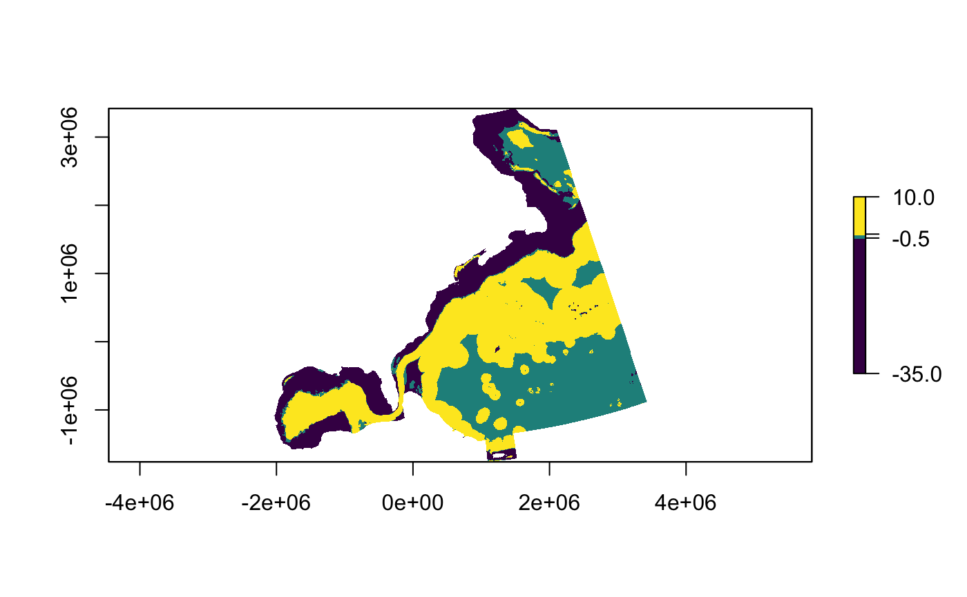
Patterns in the %N metric are broadly similar across datasets within much of the Davis Strait (to the northeast) and the Sargasso Sea (to the southeast). However, a dichotomy between extrapolation levels on and the off the continental shelf is apparent, with covariate transformations tempering extrapolation in deeper waters, at the cost of reduced confidence in extrapolations made closer to shore.