A short introduction to dsmextra
Phil J. Bouchet, David L. Miller, Jason Roberts, Laura Mannocci, Catriona M Harris, Len Thomas
Centre for Research into Ecological & Environmental Modelling, University of St Andrews2021-06-01
dsmextra.RmdPreamble
This vignette illustrates the use of the dsmextra R package for quantifying and visualising model extrapolation in environmental space. The package has its roots in density surface modelling (DSM) — as implemented in package dsm (Miller et al. 2015) — but can be easily applied to any kind of spatially-explicit ecological data. The underlying theory behind extrapolation detection is covered at length in Mesgaran et al. (2014) and King and Zeng (2007). A full description of the package is given in Bouchet et al. (2020).
dsmextra builds upon the functions available in the ecospat (Broennimann et al. 2016) and WhatIf (Gandrud et al. 2017) packages to provide user-friendly tools relevant to the analysis of ecological data, including distance sampling data. Specifically, dsmextra enables an a priori evaluation of environmental extrapolation, when using a model built in a reference system to make predictions in a separate target system (e.g., a different geographical area and/or a past/future time period) (Sequeira et al. 2018).
Here, we showcase the features of dsmextra with a case study on sperm whales (Physeter macrocephalus) in the Mid-Atlantic. The data come from two shipboard line transect surveys conducted by the National Oceanic and Atmospheric Administration (NOAA)’s Northeast and Southeast Fisheries Science Centers in 2004, and represent a subset of the survey effort shown in Roberts et al. (2016) and Mannocci et al. (2017). A basic level of familiarity with density surface modelling is assumed - for technical details, see Miller et al. (2013).
Note that the vignette accompanies a detailed technical report on extrapolation in cetacean density surface models. See Bouchet et al. (2019) for more information.
Installation
The latest development version of dsmextra can be installed from GitHub (this requires the remotes package):
remotes::install_github("densitymodelling/dsmextra", dependencies = TRUE)
The code below loads required libraries and sets some general options.
#'---------------------------------------------
# Other required libraries
#'---------------------------------------------
library(dsmextra)     # Extrapolation toolkit for ecological models
library(raster)       # Geographic data analysis and modeling
library(tidyverse)    # Packages for data science
library(magrittr)     # Pipe operator

#'--------------------------------------------------------------------
# Set tibble options
#'--------------------------------------------------------------------
options(tibble.width = Inf) # All tibble columns shown
options(pillar.neg = FALSE) # No colouring negative numbers
options(pillar.subtle = TRUE)
options(pillar.sigfig = 4)

#'--------------------------------------------------------------------
# Set knitr options
#'--------------------------------------------------------------------
knitr::opts_chunk$set(echo = TRUE)
Overview
This vignette covers all the steps required to undertake an extrapolation assessment, and explains how to:
- Quantify extrapolation using
compute_extrapolation. - Obtain a summary of extrapolation using
summary.
- Identify covariates responsible for extrapolation using
compare_covariates. - Calculate a neighbourhood metric of extrapolation using
compute_nearby. - Generate maps of extrapolation using
map_extrapolation. - Run a full assessment using
extrapolation_analysis.
The data for this example are included in dsmextra as a list containing information about both (1) the surveyed area (i.e., here, the line transects ‘chopped’ into segments) and (2) the prediction area. We refer to segs as the reference (or calibration) data/system/conditions, and to predgridas the target data/system/conditions (Sequeira et al. 2018). Note that predgrid holds the coordinates and covariate values for grid cells over which density surface model predictions are sought (although model fitting is outside the scope of this vignette).
#'---------------------------------------------
# Load and extract the data
#'---------------------------------------------
data("spermwhales")
segs <- spermwhales$segs
predgrid <- spermwhales$predgrid

#'---------------------------------------------
# Quick inspection
#'---------------------------------------------
knitr::kable(head(segs[,c(1, 3:12)]), format = "pandoc")
| Sample.Label | SegmentID | Depth | DistToCAS | SST | EKE | NPP | x | y | Effort | Survey |
|---|---|---|---|---|---|---|---|---|---|---|
| 1 | 1 | 118.5027 | 14468.1533 | 15.54390 | 0.0014443 | 1908.129 | 214544.0 | 689074.3 | 10288.91 | en04395 |
| 2 | 2 | 119.4853 | 10262.9648 | 15.88358 | 0.0014198 | 1889.540 | 222654.3 | 682781.0 | 10288.91 | en04395 |
| 3 | 3 | 177.2779 | 6900.9829 | 16.21920 | 0.0011705 | 1842.057 | 230279.9 | 675473.3 | 10288.91 | en04395 |
| 4 | 4 | 527.9562 | 1055.4124 | 16.45468 | 0.0004102 | 1823.942 | 239328.9 | 666646.3 | 10288.91 | en04395 |
| 5 | 5 | 602.6378 | 1112.6293 | 16.62554 | 0.0002553 | 1721.949 | 246686.5 | 659459.2 | 10288.91 | en04395 |
| 6 | 6 | 1094.4402 | 707.5795 | 16.83725 | 0.0006556 | 1400.281 | 254307.0 | 652547.2 | 10288.91 | en04395 |
| x | y | Depth | SST | NPP | DistToCAS | EKE | off.set | LinkID | |
|---|---|---|---|---|---|---|---|---|---|
| 126 | 547984.6 | 788254 | 153.5983 | 12.0461 | 1462.521 | 11788.974 | 0.0008 | 1e+08 | 1 |
| 127 | 557984.6 | 788254 | 552.3107 | 12.8138 | 1465.410 | 5697.248 | 0.0010 | 1e+08 | 2 |
| 258 | 527984.6 | 778254 | 96.8199 | 12.9025 | 1429.432 | 13722.626 | 0.0012 | 1e+08 | 3 |
| 259 | 537984.6 | 778254 | 138.2376 | 13.2139 | 1424.862 | 9720.671 | 0.0013 | 1e+08 | 4 |
| 260 | 547984.6 | 778254 | 505.1439 | 13.7566 | 1379.351 | 8018.690 | 0.0027 | 1e+08 | 5 |
| 261 | 557984.6 | 778254 | 1317.5952 | 14.4252 | 1348.544 | 3775.462 | 0.0046 | 1e+08 | 6 |
A quick map is useful to assess the distribution of sperm whale sightings throughout the area. (Note: the transect lines (transects) and sightings (obs) are not included in the package, but are shown here for illustrative purposes).
#'---------------------------------------------
# Create an outline of the study area boundaries
#'---------------------------------------------
study_area <- predgrid[, c("x", "y")]
study_area$value <- 1
study_area <- raster::rasterFromXYZ(study_area, crs = sp::CRS("+proj=aea +lat_1=38 +lat_2=30 +lat_0=34 +lon_0=-73 +x_0=0 +y_0=0 +datum=WGS84 +units=m +no_defs +ellps=WGS84 +towgs84=0,0,0"))
study_area <- raster::rasterToPolygons(study_area, dissolve = TRUE)
study_area <- sp::spTransform(study_area, CRSobj = sp::proj4string(transects))
study_area <- smoothr::smooth(study_area, method = "ksmooth", smoothness = 5)

#'---------------------------------------------
# Produce a simple plot
#'---------------------------------------------
plot(study_area, col = "lightskyblue1") # Region boundary
plot(transects, add = TRUE, col = "skyblue3") # Survey tracks
maps::map("world", fill = TRUE, col = "grey",
          xlim = range(obs$coords.x1),
          ylim = range(obs$coords.x2), add = TRUE)
pts <- obs # Sightings
coordinates(pts) <- ~ coords.x1 + coords.x2
axis(1); axis(2); box()
points(pts, pch = 16)
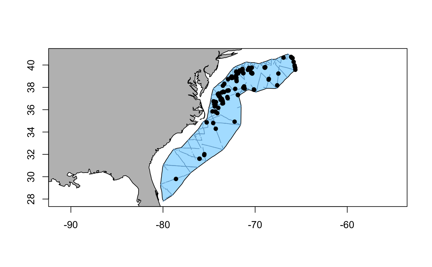
Fig. 1: Distribution of sperm whale (Physeter macrocephalus) sightings within the study area off the US East coast. Surveyed transects are shown as solid lines.
First, we define the projected coordinate system appropriate to the study area (i.e., Albers Equal Area, +proj=aea). Our explanatory covariates of interest are: seabed depth (Depth), sea surface temperature (SST), primary productivity (NPP), distance to the nearest canyons and seamounts (DistToCAS), and eddy kinetic energy (EKE) – see Roberts et al. (2016) for details.
#'---------------------------------------------
# Define projected coordinate system
#'---------------------------------------------
aftt_crs <- sp::CRS("+proj=aea +lat_1=38 +lat_2=30 +lat_0=34 +lon_0=-73 +x_0=0 +y_0=0 +datum=WGS84 +units=m +no_defs +ellps=WGS84 +towgs84=0,0,0")

#'---------------------------------------------
# Define environmental covariates of interest
#'---------------------------------------------
covariates.spermwhale <- c("Depth", "SST", "NPP", "DistToCAS", "EKE")
Quantifying extrapolation
To assess extrapolation in environmental space, we can run the extrapolation detection (ExDet) tool proposed by Mesgaran et al. (2014) using the function compute_extrapolation. Note that this tool was originally implemented in the ecospat package, although with more limited capabilities.
The following arguments are required:
-
samples: reference data -
covariate.names: names of covariates of interest -
prediction.grid: target data -
coordinate.system: projected coordinate system relevant to study location
Here, we store the results in an object called spermwhale.extrapolation. Values are expressed as both the number (n) of grid cells subject to extrapolation, and the proportion (%) of the target system that this represents.
spermwhale.extrapolation <- compute_extrapolation(samples = segs,
                                   covariate.names = covariates.spermwhale,
                                   prediction.grid = predgrid,
                                   coordinate.system = aftt_crs)
In this example, the vast majority of prediction grid cells (n = 5,175 – i.e., 97.92%) are characterised by environmental conditions (defined along the axes of the covariates specified above) similar (aka ‘analogue’) to those captured in the original sample (segs). A quick check reveals that those results align with our expectations from the data in predgrid.
# Number of cells subject to univariate extrapolation (see below for definition)
predgrid %>%
  dplyr::filter(!dplyr::between(Depth, min(segs$Depth), max(segs$Depth)) |
                  !dplyr::between(SST, min(segs$SST), max(segs$SST)) |
                  !dplyr::between(NPP, min(segs$NPP), max(segs$NPP)) |
                  !dplyr::between(DistToCAS, min(segs$DistToCAS), max(segs$DistToCAS)) |
                  !dplyr::between(EKE, min(segs$EKE), max(segs$EKE))) %>%
  nrow()
## [1] 65In practice, compute_extrapolation returns a list containing both data.frames (extrapolation values) and rasters (spatial representation of these values), with the following structure:
str(spermwhale.extrapolation, 2)
## List of 8
##  $ type             : chr [1:2] "extrapolation" "mic"
##  $ data             :List of 4
##   ..$ all          :'data.frame':    5285 obs. of  6 variables:
##   ..$ univariate   :'data.frame':    65 obs. of  6 variables:
##   ..$ combinatorial:'data.frame':    45 obs. of  6 variables:
##   ..$ analogue     :'data.frame':    5175 obs. of  6 variables:
##  $ rasters          :List of 2
##   ..$ ExDet:List of 4
##   ..$ mic  :List of 4
##  $ summary          :List of 2
##   ..$ extrapolation:List of 6
##   ..$ mic          :List of 2
##   ..- attr(*, "class")= chr [1:2] "extrapolation_results_summary" "list"
##  $ covariate.names  : chr [1:5] "Depth" "SST" "NPP" "DistToCAS" ...
##  $ samples          :'data.frame':   949 obs. of  12 variables:
##   ..$ Sample.Label: int [1:949] 1 2 3 4 5 6 7 8 9 10 ...
##   ..$ CenterTime  : Factor w/ 949 levels "2004/06/24 07:27:04",..: 1 2 3 4 5 6 7 8 9 10 ...
##   ..$ SegmentID   : int [1:949] 1 2 3 4 5 6 7 8 9 10 ...
##   ..$ Depth       : num [1:949] 119 119 177 528 603 ...
##   ..$ DistToCAS   : num [1:949] 14468 10263 6901 1055 1113 ...
##   ..$ SST         : num [1:949] 15.5 15.9 16.2 16.5 16.6 ...
##   ..$ EKE         : num [1:949] 0.001444 0.00142 0.00117 0.00041 0.000255 ...
##   ..$ NPP         : num [1:949] 1908 1890 1842 1824 1722 ...
##   ..$ x           : num [1:949] 214544 222654 230280 239329 246687 ...
##   ..$ y           : num [1:949] 689074 682781 675473 666646 659459 ...
##   ..$ Effort      : num [1:949] 10289 10289 10289 10289 10289 ...
##   ..$ Survey      : Factor w/ 2 levels "en04395","GU0403": 1 1 1 1 1 1 1 1 1 1 ...
##  $ prediction.grid  :'data.frame':   5285 obs. of  9 variables:
##   ..$ x        : num [1:5285] 547985 557985 527985 537985 547985 ...
##   ..$ y        : num [1:5285] 788254 788254 778254 778254 778254 ...
##   ..$ Depth    : num [1:5285] 153.6 552.3 96.8 138.2 505.1 ...
##   ..$ SST      : num [1:5285] 12 12.8 12.9 13.2 13.8 ...
##   ..$ NPP      : num [1:5285] 1463 1465 1429 1425 1379 ...
##   ..$ DistToCAS: num [1:5285] 11789 5697 13723 9721 8019 ...
##   ..$ EKE      : num [1:5285] 0.0008 0.001 0.0012 0.0013 0.0027 0.0046 0.0067 0.0027 0.0032 0.0055 ...
##   ..$ off.set  : num [1:5285] 1e+08 1e+08 1e+08 1e+08 1e+08 1e+08 1e+08 1e+08 1e+08 1e+08 ...
##   ..$ LinkID   : int [1:5285] 1 2 3 4 5 6 7 8 9 10 ...
##  $ coordinate.system:Formal class 'CRS' [package "sp"] with 1 slot
##  - attr(*, "class")= chr [1:2] "extrapolation_results" "list"
Three types of extrapolation can be identified (Figure 2):
-
Univariate extrapolation occurs when
ExDetvalues < 0. This is also known as mathematical, strict, or Type 1 extrapolation, and represents conditions outside the range of individual covariates in the reference sample. -
Combinatorial extrapolation occurs when
ExDetvalues > 1. This is also known as multivariate or Type 2 extrapolation, and describes novel combinations of values encountered within the univariate range of reference covariates. Such combinations are identified based on the Mahalanobis distance metric (D2), a well-known and scale-invariant measure of multivariate outliers (Rousseeuw and Zomeren 1990). - Lastly, values between 0 and 1 denote predictions made in analogue conditions. These correspond to what is commonly referred to as interpolation, although if found in a different region in space or past/future period in time, then the terms geographical/temporal extrapolation are sometimes also used.
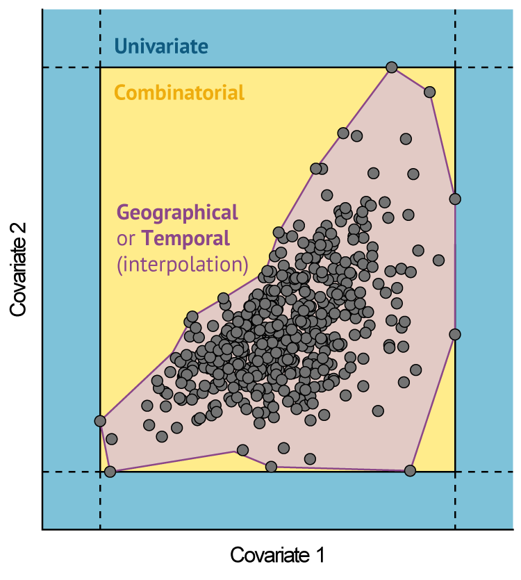
Fig. 2: Schematic representation of extrapolation in multivariate environmental space, based on two hypothetical covariates. Reference data points are represented as grey circles. Shaded areas correspond to different types of extrapolation outside the envelope of the reference data. Univariate extrapolation occurs beyond the range of individual covariates. Combinatorial extrapolation occurs within this range, but outside the reference hyperspace/hypervolume. Source: Bouchet et al. (2019), adapted from Mesgaran et al. (2014).
compute_extrapolation also determines which covariate makes the largest contribution to extrapolation for any given grid cell, i.e., the most influential covariate (mic) (Mesgaran et al. 2014). In univariate extrapolation, this is the covariate that leads to the highest negative univariate distance from the initial covariate range. In combinatorial extrapolation, this corresponds to the covariate whose omission (while retaining all others) makes the largest reduction in the Mahalanobis distance to the centroid of the reference data. See Mesgaran et al. (2014) for formulae and technical explanations.
ExDet values can be retrieved from the returned list, as below:
# Example from combinatorial extrapolation
head(spermwhale.extrapolation$data$combinatorial)
##          x      y    ExDet mic_univariate mic_combinatorial mic
## 1 557984.6 728254 1.106042             NA                 3   3
## 2 567984.6 728254 1.090527             NA                 3   3
## 3 577984.6 728254 1.447405             NA                 3   3
## 4 587984.6 728254 1.437475             NA                 3   3
## 5 607984.6 728254 1.186687             NA                 3   3
## 6 527984.6 718254 1.240072             NA                 3   3
Summarising extrapolation
compute_extrapolation also generates a summary table, which can be printed as follows:
summary(spermwhale.extrapolation)
##
##
## Table: Extrapolation
##
## Type            Count         Percentage
## --------------  ------------  ------------
## Univariate      65            1.23
## Combinatorial   45            0.85
## -----------     -----------   -----------
## Sub-total       110           2.08
## -----------     -----------   -----------
## Analogue        5175          97.92
## -----------     -----------   -----------
## Total           5285          100
##
##
## Table: Most influential covariates (MIC)
##
## Type            Covariate     Count         Percentage
## --------------  ------------  ------------  ------------
## Univariate      EKE           24            0.45
## Univariate      SST           17            0.32
## Univariate      Depth         16            0.3
## Univariate      NPP           6             0.11
## Univariate      DistToCAS     2             0.038
## -----------     -----------   -----------   -----------
## Sub-total                     65            1.2
## -----------     -----------   -----------   -----------
## Combinatorial   NPP           39            0.74
## Combinatorial   Depth         6             0.11
## -----------     -----------   -----------   -----------
## Sub-total                     45            0.85
## -----------     -----------   -----------   -----------
## Total                         110           2.1
Comparing covariates
The extent and magnitude of extrapolation naturally vary with the type and number of covariates considered. It may be useful, therefore, to test different combinations of covariates to inform their selection a priori, i.e., before model fitting, to support model parsimony.
The compare_covariates function is available for this purpose. It is designed to assess extrapolation iteratively for all combinations of n.covariates, and returns an overview of those that minimise/maximise extrapolation (as measured by the number of grid cells subject to extrapolation in the prediction area).
n.covariates can be supplied as any vector of integers from 1 to p, where p is the total number of covariates available. Its default value of NULL is equivalent to 1:p, meaning that all possible combinations are tested, unless otherwise specified.
Additional arguments include:
-
extrapolation.type: one of'univariate','combinatorial'or'both' -
extrapolation.object: output list object returned bycompute_extrapolation. -
create.plots: ifTRUE, generates boxplots of results -
display.percent: ifTRUE, the y-axis of the boxplots is expressed as a percentage of the total number of grid cells inprediction.grid
Optionally, one can bypass compute_extrapolation and run this function directly by specifying the following arguments and leaving extrapolation.object set as NULL:
-
samples: reference data -
covariate.names: names of covariates of interest -
prediction.grid: target data -
coordinate.system: projected coordinate system relevant to study location
Below is an example for both types of extrapolation (univariate and combinatorial), and the full set of five covariates.
compare_covariates(extrapolation.type = "both",
                   extrapolation.object = spermwhale.extrapolation,
                   n.covariates = NULL,
                   create.plots = TRUE,
                   display.percent = TRUE)
## Preparing the data ...## Computing ...## ## Creating summaries ...## Done!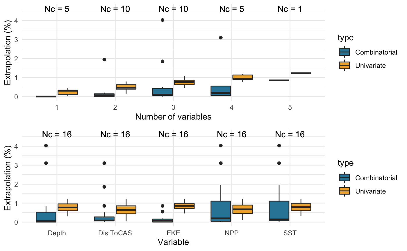
##
##
## Extrapolation   Minimum             n_min  Maximum                           n_max
## --------------  -----------------  ------  --------------------------------  ------
## Univariate      DistToCAS               2  Depth, SST, NPP, DistToCAS, EKE   65
## Combinatorial   Depth                   0  Depth, SST, NPP                   213
##                 SST                     0  -                                 -
##                 NPP                     0  -                                 -
##                 DistToCAS               0  -                                 -
##                 EKE                     0  -                                 -
##                 Depth, DistToCAS        0  -                                 -
##                 Depth, EKE              0  -                                 -
##                 NPP, DistToCAS          0  -                                 -
##                 NPP, EKE                0  -                                 -
##                 Depth, SST, EKE         0  -                                 -
##                 Depth, NPP, EKE         0  -                                 -
## Both            DistToCAS               2  Depth, SST, NPP                   252
The top graph summarises the extent of univariate (yellow) and combinatorial (blue) extrapolation for all combinations of \(1, 2, ..., n\) covariates. The total number of combinations is given above each boxplot as \(N_c\). As expected, univariate extrapolation increases with the number of covariates considered.
The bottom graph displays the same results, summarised by covariate of interest. This may help identify any covariates that consistently lead to extrapolation, and should be avoided. Here, none of the covariates stand out as driving extrapolation more than any others, although combinatorial extrapolation is marginally more prevalent with NPP and SST.
Finding nearby data
While extrapolation is often seen as a binary concept (i.e., it either does or does not take place), it is reasonable to expect that predictions made at target points situated just outside the sampled environmental space may be more reliable than those made at points far outside it. The ExDet tool available through compute_extrapolation inherently quantifies this notion of ‘distance’ from the envelope (solid line) of the reference data (grey circles) (Figure 3A).
However, the multivariate distribution of reference data points is often far from homogeneous. It is possible, therefore, for target points representing analogue conditions to fall within sparsely sampled regions of the reference space; or conversely, for two target points reflecting an equal degree of extrapolation to have very different amounts of reference data within their vicinity (Virgili et al. 2017; Mannocci et al. 2018).
An example of this is shown in Figure 3B, where three target points \(x_1\), \(x_2\) and \(x_3\) are located equally close to the envelope of the reference data. In essence, these reflect identical degrees of extrapolation, as defined under the ExDet framework. However, given the shape of the data cloud in multivariate space, it is clear that predictions made at target point \(x_1\) will far ‘better informed’ by the sample than those made at \(x_2\) or \(x_3\), as a bigger cluster of reference points lies in their vicinity (green circle around \(x_1\)).
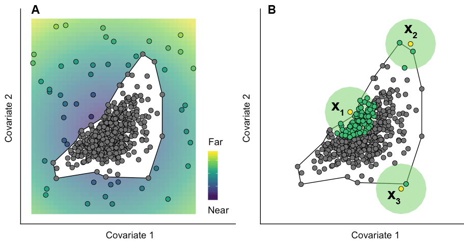
Fig. 3: Conceptual representation of two key extrapolation metrics. (A) Distance from the sampled environmental space. A target point far from the envelope of the reference data (eg. falling in the yellow area) is arguably ‘more of an extrapolation’ than one close to it (eg. falling in the purple area). (B) Neighbourhood (syn. percentage of data nearby). Due to the shape of the reference data cloud, the amount of sample information available to ‘inform’ predictions made at target points can vary considerably. Source: Bouchet et al. (2019).
The notion of neighbourhood (or percentage/proportion of data nearby, hereafter %N) captures this very idea, and provides an additional measure of the reliability of extrapolations in multivariate environmental space (Virgili et al. 2017; Mannocci et al. 2018). In practice, %N for any target point is taken as the proportion of reference data within a radius of one geometric mean Gower’s distance (G2, calculated between all pairs of reference points) of that point (King and Zeng 2007). The Gower’s distance between two points \(i\) and \(j\) defined along the axes of \(K\) covariates is calculated as the average absolute distance between the values of these two points in each dimension, divided by the range of the data, such that:
\[G_{ij}^2=\frac{1}{K}\sum_{k=1}^{K}\frac{\left|x_{ik}-x_{jk}\right|}{\textrm{max}(X_k)-\textrm{min}(X_k)}\]
The compute_nearby function is adapted from the code given in Mannocci et al. (2018), and allows the calculation of Gower’s distances (G2) as a basis for defining the neighbourhood.
The nearby argument to this function corresponds to the radius within which neighbouhood calculations will occur. It has a default value of 1, as per Mannocci et al. (2018) and Virgili et al. (2017). Increasing its value (e.g., to say, 2) would mean doubling the size of the green circles in Figure 3B, and would lead to larger percentages of data nearby per target point.
Important: The sperm whale dataset used here is sufficiently small that compute_nearby should run in a matter of seconds on most machines. However, applying the function to larger datasets may burn out memory allocation and lead to an R session failure. Additional arguments can be passed to compute_nearby to accommodate such ‘big’ data. Their use is unnecessary here, but further details can be found in the package documentation.
#'---------------------------------------------
# Calculate Gower's distances and %N
#'---------------------------------------------
spermwhale.nearby <- compute_nearby(samples = segs,
                                    prediction.grid = predgrid,
                                    coordinate.system = aftt_crs,
                                    covariate.names = covariates.spermwhale,
                                    nearby = 1)
## Preprocessing data ...## Calculating distances ....## Calculating the geometric variance...## Calculating cumulative frequencies ...## Finishing up ...## Done!Visualising extrapolation
Lastly, we can use the map_extrapolation function to create a series of interactive html maps of extrapolation in the prediction area.
Arguments to this function are identical to those of compute_extrapolation, with the exception of:
-
map.type: output to be shown on the map. One of'extrapolation'for a map of extrapolation values,'mic'for a map of the most influential covariates, or'nearby'for a neighbourhood map (proportion of reference data near each target grid cell, a.k.a%N). -
extrapolation.object: output object fromcompute_extrapolationorcompute_nearby.
sightings and tracks are optional arguments, and only plotted if specified. If either is provided as a matrix, then coordinates must be labelled x and y, lest a warning be returned. Tracks can also be given as a SpatialLinesDataFrame object. The resulting maps can be panned, zoomed, and all layers toggled on and off independently. However, note that maps rely on the leaflet package (Cheng et al. 2018), and thus require an internet connection; they will not work offline. Facilities to save map tiles locally for offline viewing are currently not implemented but may be rolled into a future version of the code. Finally, note that prediction.grid is only used here to set the map extent when plotting.
#'---------------------------------------------
# Rename coordinates and convert to SpatialPointsdf
#'---------------------------------------------
obs.sp <- obs %>%
  dplyr::rename(., x = coords.x1, y = coords.x2) %>%
  sp::SpatialPointsDataFrame(coords = cbind(.$x, .$y), data = ., proj4string = sp::CRS("+proj=longlat +datum=WGS84 +no_defs +ellps=WGS84 +towgs84=0,0,0")) %>%
  sp::spTransform(., CRSobj = aftt_crs)
Here’s a map of extrapolation (ExDet) values:
map_extrapolation(map.type = "extrapolation",
                  extrapolation.object = spermwhale.extrapolation,
                  sightings = obs.sp,
                  tracks = transects)
Most influential covariates (MIC):
map_extrapolation(map.type = "mic",
                  extrapolation.object = spermwhale.extrapolation,
                  sightings = obs.sp,
                  tracks = transects)
Proportion of data nearby (%N):
map_extrapolation(map.type = "nearby",
                  extrapolation.object = spermwhale.nearby,
                  sightings = obs.sp,
                  tracks = transects)
Full analysis
For simplicity, all the above analyses can be performed in a single step by calling the wrapper function extrapolation_analysis. Most arguments are derived from the individual functions presented above, and should thus be self-explanatory. Note, however, that specific parts of the analysis can be run/bypassed using the following arguments:
-
compare.covariates= ifTRUE, runcompare_covariates -
nearby.compute= ifTRUE, runcompute_nearby -
map.generate= ifTRUE, runmap_extrapolation
#'---------------------------------------------
# One function to rule them all, one funtion to find them,
# One function to bring them all, and in the darkness bind them.
#'---------------------------------------------
spermwhale.analysis <- extrapolation_analysis(samples = segs,
                                          covariate.names = covariates.spermwhale,
                                          prediction.grid = predgrid,
                                          coordinate.system = aftt_crs,
                                          compare.covariates = TRUE,
                                          compare.extrapolation.type = "both",
                                          compare.n.covariates = NULL,
                                          compare.create.plots = TRUE,
                                          compare.display.percent = TRUE,
                                          nearby.compute = TRUE,
                                          nearby.nearby = 1,
                                          map.generate = TRUE,
                                          map.sightings = obs.sp,
                                          map.tracks = transects)
Results are packaged in a list object with three levels, i.e., extrapolation, nearby, and maps, representing the outputs of each step in the analysis.
Conclusion
This vignette has outlined the steps need to quantify extrapolation in environmental space using the dsmextra R package. Note that many possible models (and model types) can be fitted to distance sampling or related data, each potentially behaving differently outside reference conditions for any given level of extrapolation (Yates et al. 2018). Because of this, the tools presented herein are model-agnostic and only designed to provide an a priori assessment. This may, in turn, help inform modelling decisions and model interpretations, but caution should always be exercised when performing model selection, discrimination and criticism.