A priori covariate selection using dsmextra
Phil J. Bouchet, David L. Miller, Jason Roberts, Laura Mannocci, Catriona M Harris, Len Thomas
Centre for Research into Ecological & Environmental Modelling, University of St Andrews2021-06-01
dsmextra-covariateselection.RmdPreamble
This vignette demonstrates how dsmextra can be used to guide covariate selection a priori, before model fitting. Full details on the case study can be found in the Supplementay Material accompanying Bouchet et al. (2020).
Installation
The latest development version of dsmextra can be installed from GitHub (this requires the remotes package):
remotes::install_github("densitymodelling/dsmextra", dependencies = TRUE)
The code below loads required libraries and sets some general options.
#'---------------------------------------------
# Other required libraries
#'---------------------------------------------
library(dsm)                  # Density surface modelling of distance sampling data
library(dsmextra)             # Extrapolation toolkit for ecological models
library(Distance)             # Distance sampling detection function and abundance estimation
library(raster)               # Geographic data analysis and modelling
library(tidyverse)            # Tools and functions for data science
library(sf)                   # Simple features in R
library(magrittr)            # Code semantics
library(GGally)               # Extension to ggplot2
library(viridisLite)          # Default Color Maps from 'matplotlib'
library(smoothr)              # Smooth and tidy spatial features
library(sp)                   # Classes and methods for spatial data

set.seed(42) # Set the random seed

#'---------------------------------------------
# Set tibble options
#'---------------------------------------------
options(tibble.width = Inf) # All tibble columns shown
options(pillar.neg = FALSE) # No colouring negative numbers
options(pillar.subtle = TRUE)
options(pillar.sigfig = 4)

#'---------------------------------------------
# Set knitr options
#'---------------------------------------------
knitr::opts_chunk$set(echo = TRUE)

#'---------------------------------------------
# Set ggplot2 options
#'---------------------------------------------
gg.opts <- theme(panel.grid.minor = element_blank(),
                 panel.background = element_blank(),
                 plot.title = element_text(size = 13, face = "bold"),
                 legend.title = element_text(size = 12),
                 legend.text = element_text(size = 11),
                 axis.text = element_text(size = 11),
                 panel.grid.major = element_line(colour = 'lightgrey', size = 0.1),
                 axis.title.x = element_blank(),
                 axis.title.y = element_blank(),
                 legend.position = "bottom")

#'---------------------------------------------
# Geographic coordinate systems
#'---------------------------------------------
latlon_proj <- sp::CRS("+proj=longlat +datum=WGS84 +ellps=WGS84 +towgs84=0,0,0")
aftt_proj <- sp::CRS("+proj=aea +lat_1=40.66666666666666 +lat_2=27.33333333333333 +lat_0=34 +lon_0=-78 +x_0=0 +y_0=0 +datum=WGS84 +units=m +no_defs +ellps=WGS84 +towgs84=0,0,0")
GulfMexico_proj <- sp::CRS("+proj=lcc +lat_1=20 +lat_2=60 +lat_0=40 +lon_0=-96 +x_0=0 +y_0=0 +ellps=GRS80 +datum=NAD83 +units=m +no_defs ")
Data
The data and custom functions required to run this example can be downloaded as a ZIP archive from the Supplementary Information section of Bouchet et al. (2020), available at https://besjournals.onlinelibrary.wiley.com/doi/abs/10.1111/2041-210X.13469. The below assumes that the data files have been saved in the working directory.
The environmental covariates of interest include:
- Bathymetric depth [static]
- Seabed slope [static]
- Distance to the coast [static]
- Distance to the nearest submarine canyon or seamount [static]
- Current speed [dynamic]
- Sea surface temperature [dynamic]
Note that for simplicity, dynamic covariates were summarised as a yearly median across 12 monthly rasters. Note also that the raster stack in covariates.rda also contains layer representing the surface area of each grid cell. This will be useful when making predictions from density surface models, which include an offset term for the area effectively surveyed.
#'---------------------------------------------
# Load the covariate rasters
#'---------------------------------------------
load("covariates.rda")

#'---------------------------------------------
# Create the final prediction data.frame
#'---------------------------------------------
pred.grid <- raster::stack(env.rasters) %>%
  raster::projectRaster(from = ., crs = GulfMexico_proj) %>%
  raster::as.data.frame(., xy = TRUE) %>%
  na.omit()
## Warning in wkt(projfrom): CRS object has no comment## Warning in wkt(pfrom): CRS object has no comment## Warning in rgdal::rawTransform(projfrom, projto, nrow(xy), xy[, 1], xy[, : Using
## PROJ not WKT2 strings## Warning in rgdal::rawTransform(fromcrs, crs, nrow(xy), xy[, 1], xy[, 2]): Using
## PROJ not WKT2 strings## Warning in rgdal::rawTransform(projto_int, projfrom, nrow(xy), xy[, 1], : Using
## PROJ not WKT2 strings#'--------------------------------------------- # Retrieve covariate values for each segment #'--------------------------------------------- survey.segdata <- raster::projectRaster(from = raster::stack(env.rasters), crs = GulfMexico_proj) %>% raster::extract(x = ., y = sp::SpatialPointsDataFrame(coords = survey.segdata[, c("x", "y")], data = survey.segdata, proj4string = GulfMexico_proj), sp = TRUE) %>% raster::as.data.frame(.) %>% dplyr::select(-c(x.1, y.1))
## Warning in wkt(projfrom): CRS object has no comment## Warning in wkt(pfrom): CRS object has no comment## Warning in rgdal::rawTransform(projfrom, projto, nrow(xy), xy[, 1], xy[, : Using
## PROJ not WKT2 strings## Warning in rgdal::rawTransform(fromcrs, crs, nrow(xy), xy[, 1], xy[, 2]): Using
## PROJ not WKT2 strings## Warning in rgdal::rawTransform(projto_int, projfrom, nrow(xy), xy[, 1], : Using
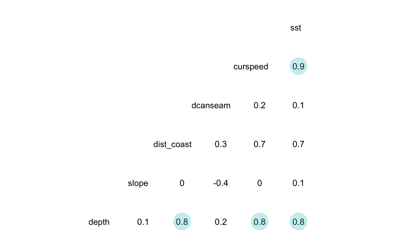
## PROJ not WKT2 strings#'--------------------------------------------- # Check collinearity between covariates #'--------------------------------------------- survey.segdata[, names(env.rasters)[1:6]] %>% GGally::ggcorr(., geom = "blank", label = TRUE, hjust = 0.75, method = c('complete.obs', 'pearson')) + geom_point(size = 10, aes(color = coefficient > 0, alpha = abs(coefficient) > 0.7)) + scale_alpha_manual(values = c("TRUE" = 0.25, "FALSE" = 0)) + guides(color = FALSE, alpha = FALSE)
Extrapolation assessment
# Define environmental covariates of interest
stenella.covariates <- names(env.rasters)[1:6]

# Univariate + combinatorial extrapolation (ExDet)
stenella.exdet <- dsmextra::compute_extrapolation(samples = survey.segdata,
                                                  covariate.names = stenella.covariates,
                                                  prediction.grid = pred.grid,
                                                  coordinate.system = GulfMexico_proj)
## Computing ...## Done!summary(stenella.exdet)
##
##
## Table: Extrapolation
##
## Type Count Percentage
## -------------- ------------ ------------
## Univariate 7515 48.13
## Combinatorial 2178 13.95
## ----------- ----------- -----------
## Sub-total 9693 62.08
## ----------- ----------- -----------
## Analogue 5921 37.92
## ----------- ----------- -----------
## Total 15614 100
##
##
## Table: Most influential covariates (MIC)
##
## Type Covariate Count Percentage
## -------------- ------------ ------------ ------------
## Univariate sst 2693 17
## Univariate depth 2536 16
## Univariate dcanseam 1415 9.1
## Univariate dist_coast 557 3.6
## Univariate curspeed 196 1.3
## Univariate slope 118 0.76
## ----------- ----------- ----------- -----------
## Sub-total 7515 48
## ----------- ----------- ----------- -----------
## Combinatorial depth 1633 10
## Combinatorial slope 503 3.2
## Combinatorial curspeed 28 0.18
## Combinatorial sst 7 0.045
## Combinatorial dist_coast 5 0.032
## Combinatorial dcanseam 2 0.013
## ----------- ----------- ----------- -----------
## Sub-total 2178 14
## ----------- ----------- ----------- -----------
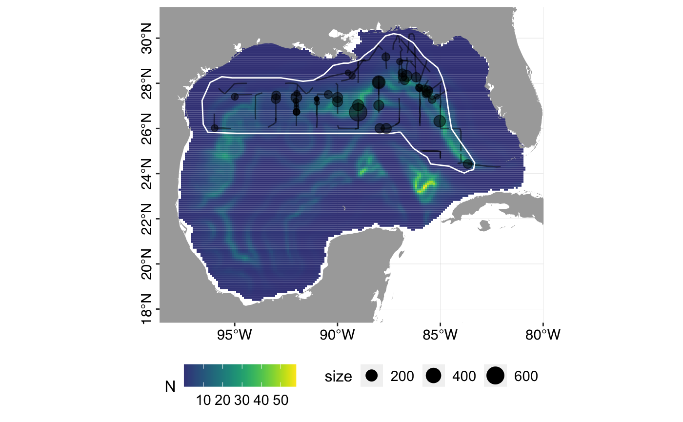
## Total 9693 62# Percentage of data nearby (%N) stenella.nearby <- dsmextra::compute_nearby(samples = survey.segdata, covariate.names = stenella.covariates, prediction.grid = pred.grid, nearby = 1, coordinate.system = GulfMexico_proj)
## Preprocessing data ...## Calculating distances ....## Calculating the geometric variance...## Calculating cumulative frequencies ...## Finishing up ...## Done!# Maps # (1) Univariate + combinatorial extrapolation (ExDet) dsmextra::map_extrapolation(map.type = "extrapolation", extrapolation.object = stenella.exdet)
## Warning in dsmextra::map_extrapolation(map.type = "extrapolation",
## extrapolation.object = stenella.exdet): map_extrapolation relies on the leaflet
## package, which is built around a Web Mercator projection (EPSG:3857), and
## therefore requires rasters to be reprojected for plotting. As a result, minor
## discrepancies may occur between the interactive maps shown in the viewer, and
## the underlying raw data. The latter can be accessed directly from extrapolation
## object returned by <compute_extrapolation> and visualised using alternative
## packages such as ggplot2.
# (2) Most influential covariates (MIC) dsmextra::map_extrapolation(map.type = "mic", extrapolation.object = stenella.exdet, base.layer = "gray")
## Warning in dsmextra::map_extrapolation(map.type = "mic", extrapolation.object
## = stenella.exdet, : map_extrapolation relies on the leaflet package, which
## is built around a Web Mercator projection (EPSG:3857), and therefore requires
## rasters to be reprojected for plotting. As a result, minor discrepancies may
## occur between the interactive maps shown in the viewer, and the underlying raw
## data. The latter can be accessed directly from extrapolation object returned
## by <compute_extrapolation> and visualised using alternative packages such as
## ggplot2.
# (3) Percentage of data nearby (%N) dsmextra::map_extrapolation(map.type = "nearby", extrapolation.object = stenella.nearby)
## Warning in dsmextra::map_extrapolation(map.type = "nearby", extrapolation.object
## = stenella.nearby): map_extrapolation relies on the leaflet package, which
## is built around a Web Mercator projection (EPSG:3857), and therefore requires
## rasters to be reprojected for plotting. As a result, minor discrepancies may
## occur between the interactive maps shown in the viewer, and the underlying raw
## data. The latter can be accessed directly from extrapolation object returned
## by <compute_extrapolation> and visualised using alternative packages such as
## ggplot2.
# Compare the extent of univariate and combinatorial extrapolation # (ExDet metric) associated with different combinations of covariates dsmextra::compare_covariates(extrapolation.type = "both", extrapolation.object = stenella.exdet, n.covariates = NULL, # All possible combinations create.plots = TRUE, display.percent = TRUE)
## Preparing the data ...## Computing ...## ## Creating summaries ...## Done!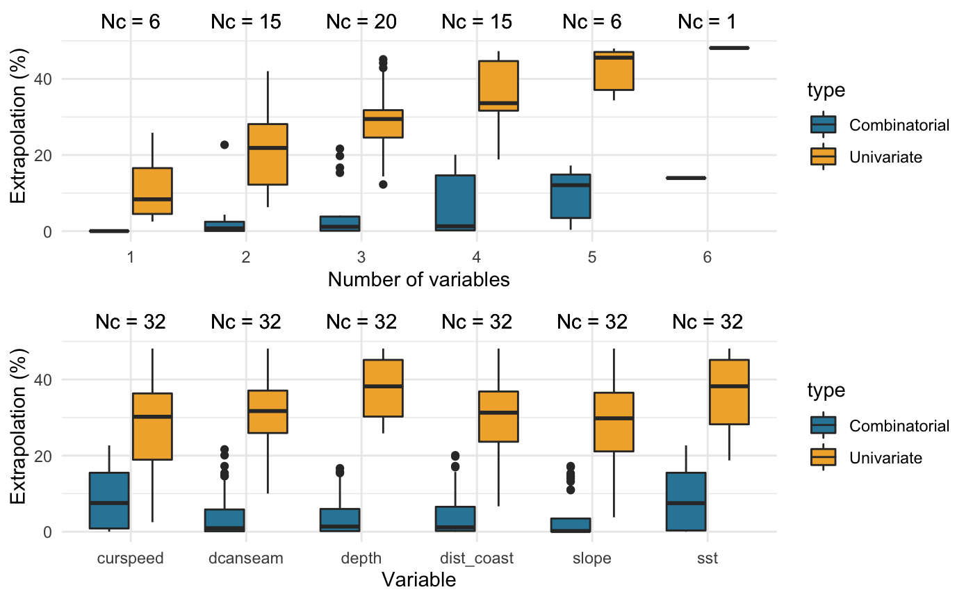
##
##
## Extrapolation   Minimum       n_min  Maximum                                             n_max
## --------------  -----------  ------  --------------------------------------------------  ------
## Univariate      curspeed        392  depth, slope, dist_coast, dcanseam, curspeed, sst   7515
## Combinatorial   depth             0  curspeed, sst                                       3541
##                 slope             0  -                                                   -
##                 dist_coast        0  -                                                   -
##                 dcanseam          0  -                                                   -
##                 curspeed          0  -                                                   -
##                 sst               0  -                                                   -
## Both            curspeed        392  depth, dist_coast, dcanseam, curspeed, sst          9812
Density surface model
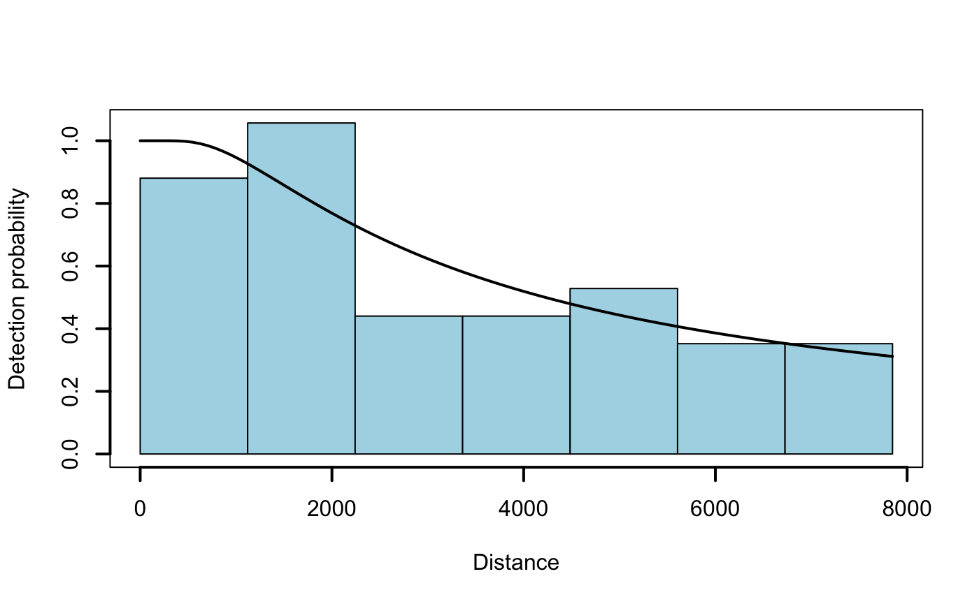
# Fit a simple hazard-rate detection model to the distance data (no covariates)
detfc.hr.null <- Distance::ds(data = distdata, truncation = max(distdata$distance),
                              key = "hr", adjustment = NULL)
## Fitting hazard-rate key function## Key only model: not constraining for monotonicity.## AIC= 841.253## No survey area information supplied, only estimating detection function.# Plot the fitted model on top of a histogram of distances plot(detfc.hr.null, showpoints = FALSE, lwd = 2, pl.col = "lightblue")
# Create model formulae with and without chosen covariates

dsm.formulas <- make_formulas(remove.covariates = c("depth", "sst"))

# Fit the two competing density surface models: 0 (all covariates), 1 (filtered set)
dsm.0 <- dsm::dsm(formula = dsm.formulas$f0,
                  ddf.obj = detfc.hr.null,
                  segment.data = survey.segdata,
                  observation.data = obsdata,
                  method = "REML",
                  family = tw())

dsm.1 <- dsm::dsm(formula = dsm.formulas$f1,
                  ddf.obj = detfc.hr.null,
                  segment.data = survey.segdata,
                  observation.data = obsdata,
                  method = "REML",
                  family = tw())

AIC(dsm.0, dsm.1) # AIC scores
##             df      AIC
## dsm.0 21.19301 850.0096
## dsm.1 17.79570 858.5654
# Perform residual checks model_checks(dsm.0) model_checks(dsm.1)
# Model predictions
dsm.0.pred <- predict(object = dsm.0, pred.grid, pred.grid$area)
dsm.1.pred <- predict(object = dsm.1, pred.grid, pred.grid$area)

# Abundance estimates
sum(dsm.0.pred); sum(dsm.1.pred)
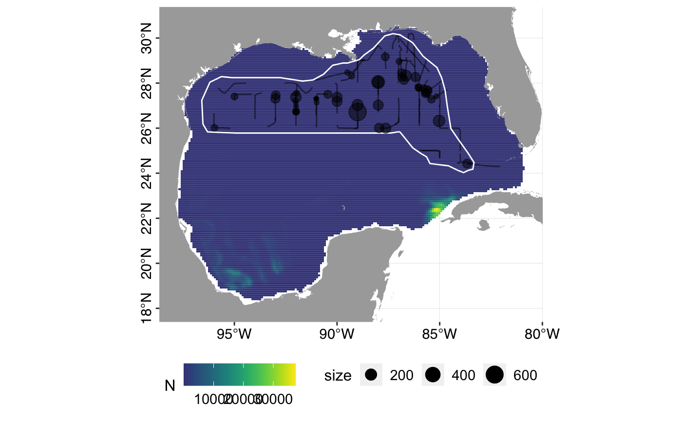
## [1] 4258441## [1] 59320.63# Variance estimation - there are no covariates in the detection function # so we use dsm.var.gam rather than dsm.var.prop # The below code may take several minutes, so is commented out. # varsplit <- split(pred.grid, 1:nrow(pred.grid)) # dsm.0.var <- dsm::dsm.var.gam(dsm.obj = dsm.0, pred.data = varsplit, off.set = pred.grid$area) # dsm.1.var <- dsm::dsm.var.gam(dsm.obj = dsm.1, pred.data = varsplit, off.set = pred.grid$area) # summary(dsm.0.var) # summary(dsm.1.var) # Plot predicted density surfaces plot_predictions(dsm.predictions = dsm.0.pred)
plot_predictions(dsm.predictions = dsm.1.pred)
# Plot uncertainty surfaces
# plot_uncertainty(varprop.output = dsm.0.var, cutpoints = c(0,1,1.5,2,3,4))
# plot_uncertainty(varprop.output = dsm.1.var, cutpoints = c(0,1,1.5,2,3,4))